

Environment
Summary
This collection of data includes the following indicators, dates, and sources:
Land Use
urban/developed km2, 1992-2100, USGS
forest km2, 1992-2100 & 1982-2012, USGS & USDA
forest (mil hectares), 2010-2030(2100), Pardee
deforestation (mil hectares), 2010-2100, Pardee
cropland km2, 1992-2100 & 1982-2012, USGS & USDA
grassland/shrubland km2, 1992-2100 & 1982-2012, USGS & USDA
hay/pasture km2, 1992-2100 & 1982-2012, USGS & USDA
wetland km2, 1992-2100, USGS
Conservation Reserve Program, 1985-2012, USDA
agricultural demand (mil met tons), 2010-2030(2100), Pardee
agricultural productions (mil met tons), 2010-2030(2100), Pardee
yield in agriculture (tons/hectar), 2010-2030(2100), Pardee
Air Quality
carbon emissions from fossil fuels (bil tons), 2010-2100, Pardee
carbon emissions cumulative change (bil tons), 2010-2100, Pardee
Water Use
water usage (cubic Km), 2010-2030(2100), Pardee
water use cumulative change (cubic Km), 2010-2100, Pardee
Mining
active mines, 2004-2013, CDC
Climate Change
max temperatures, 1950-2099, USGS
precipitation, 1950-2099, USGS
snowpack, 1950-2099, USGS
soil water storage, 1950-2099, USGS
sea-level rise, 1800-2100, NCA citing Kemp, Church, Narem, Parris, Etheridge
sea-level warming, 1900-2010, NCA citing Chavez, Etheridge
extreme precipitation events, 1900-2000, NCA citing Kunkel
water demand change, 2005/2060, NCA citing Brown
water supply risk, 2050, NCA citing Roy et al.
atmospheric carbon dioxide, 1900-2000, NCA citing Etheridge
sea surface pH, 1900-2000, NCA citing Etheridge
Northeaster fisheries shifting north, 1970-2010, NCA citing Pinsky and Fogarty
Findings
Land Use
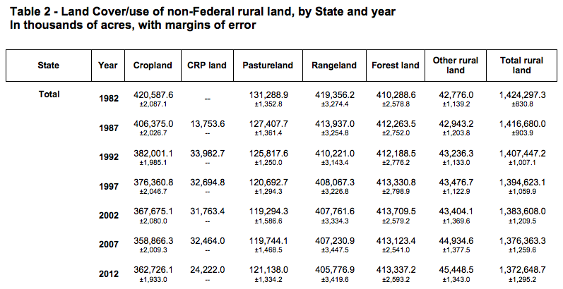
The U.S. Geological Survey tracks and forecasts several categories of land use, with charts and maps showing change under four different scenarios from 1992 through 2100. The land-use categories include acreage that is 1) urban/developed, 2) forest, 3) cropland, 4) grassland/shrubland, 5) hay/pasture, and 6) wetland.
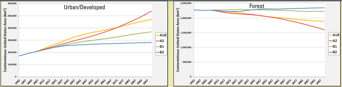
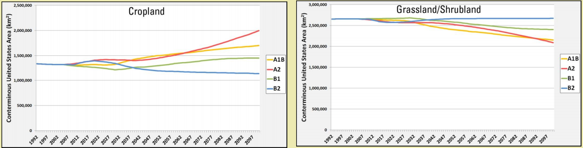
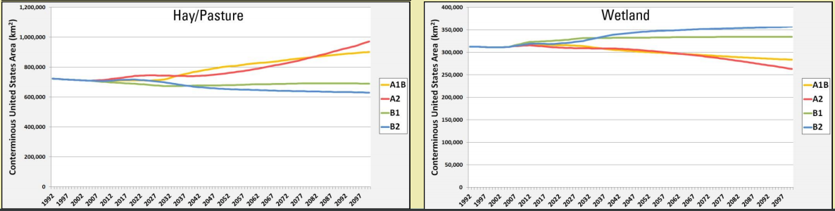
img src:
Terry Sohl, et al. December 2012.
“The Completion of Four Spatially Explicit Land-use and Land-cover (LULC) Scenarios for the Conterminous United States.” P.28
U.S. Geological Survey.
*
The USDA’s National Resources Conservation Service (NRCS) has published a periodic National Resources Inventory (NRI) since 1977, with data being collected annually since 2000. The contemporary reports give acreage counts for non-Federal lands, including cropland, Conservation Reserve Program lands, pastureland, rangeland, forest land, and other rural land.
Excerpts:
Table 2 – Land Cover/use of non-Federal rural land, 1982-2012 (quinquennial)
In thousands of acres, with margins of error
Note: Acreages for Conservation Reserve Program (CRP) land are established through geospatial processes and administrative records; therefore, statistical margins of error are not applicable and shown as a dashed line (–). CRP was not implemented until 1985.
Table 9 – Changes in land cover/use between 1982 and 2012
In thousands of acres, with margins of error
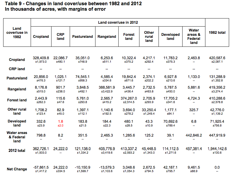
Similar tables for five-year intervals within the 1982-2012 are also presented in the report (pp.41-46).
Cropland
A land cover/use category that includes areas used for the production of adapted crops for harvest. Two subcategories of cropland are recognized: cultivated and noncultivated. Cultivated land comprises land in row crops or close-grown crops and also other cultivated cropland; for example, hayland or pastureland that is in a rotation with row or close-grown crops. Noncultivated cropland includes permanent hayland and horticultural cropland.
Pastureland
A land cover/use category of land managed primarily for the production of introduced forage plants for livestock grazing. Pastureland cover may consist of a single species in a pure stand, a grass mixture, or a grass-legume mixture. Management usually consists of cultural treatments: fertilization, weed control, reseeding, renovation, and control of grazing. For the NRI, includes land that has a vegetative cover of grasses, legumes, and/or forbs, regardless of whether or not it is being grazed by livestock.
Rangeland
A broad land cover/use category on which the climax or potential plant cover is composed
principally of native grasses, grasslike plants, forbs or shrubs suitable for grazing and browsing, and introduced forage species that are managed like rangeland. This would include areas where introduced hardy and persistent grasses, such as crested wheatgrass, are planted and such practices as deferred grazing, burning, chaining, and rotational grazing are used, with little or no chemicals or fertilizer being applied. Grasslands, savannas, many wetlands, some deserts, and tundra are considered to be rangeland. Certain communities of low forbs and shrubs, such as mesquite, chaparral, mountain shrub, and pinyon-juniper, are also included as rangeland.
src:
USDA, August 2015.
“2012 National Resources Inventory: Summary Report.”
pp. 3-2, 3-39, 3-47, 4-1
*
For projected data on farmlands, 2014-2025, see the “Crop Acreage” section of the Food research round-up, citing “USDA Agricultural Projections to 2025.”
*
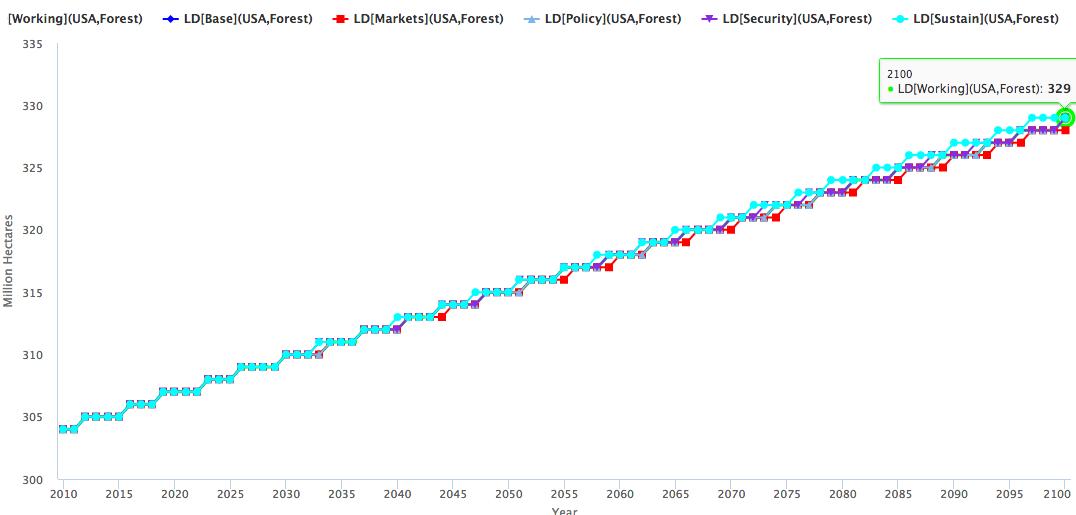
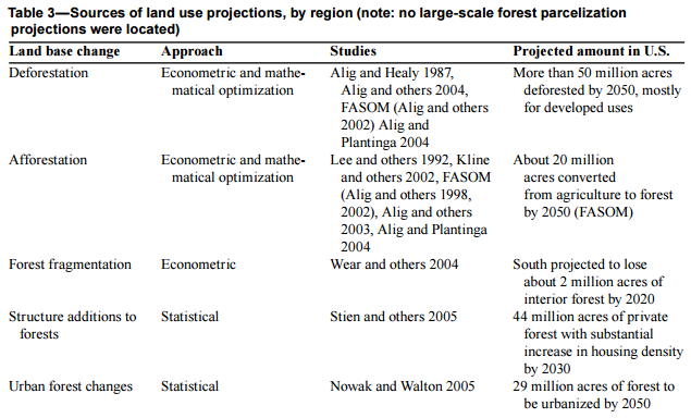
International Futures is a forecasting platform developed by Barry Hughes, based at the Pardee Center at the University of Denver. Among its many forecasts are a small set of agriculture and environment indicators.
Excerpt:
Quinquennial agriculture and environment indicators, United States, Working File
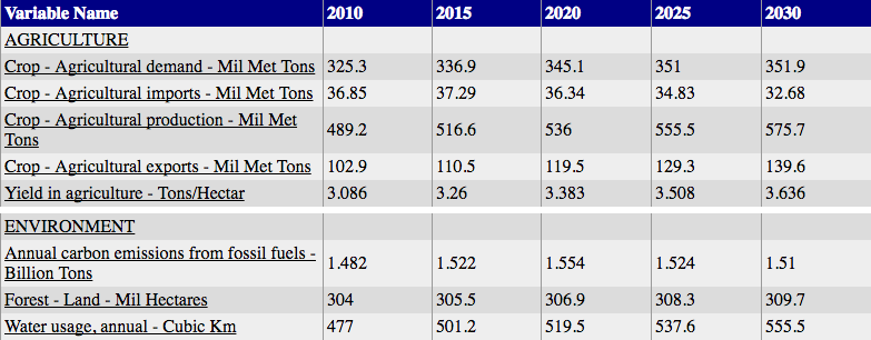
Forecast data through 2100 is available at the site for each indicator, if you click through. For example, here’s the chart for millions of hectares of forest land through 2100:
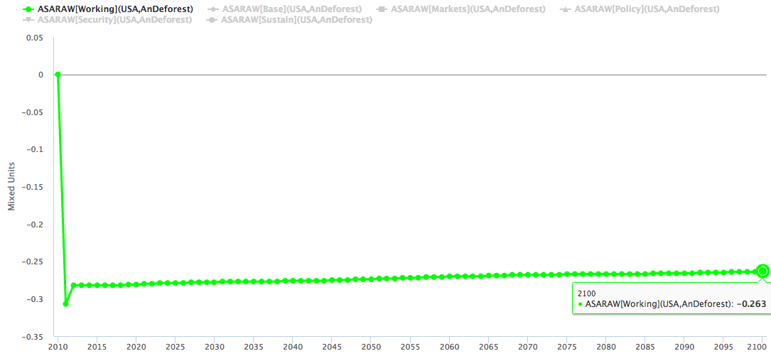
The charting tools offer several options, including specialized displays for particular issues. For example, the Advanced Sustainability Analysis, which calculates fossil fuel use, carbon emissions, deforestation, and water use in terms of intensity per million GDP, thousand population, and thousand labor. These calculations are also forecast through 2100, accessible by changing the “select year” parameter of the display.
Raw annual deforestation (million hectares), 2010-2100 (via the Advanced Sustainability Analysis table):
TO DO: EXTRACT ANNUAL DATA POINTS BY CLICKING THROUGH ON THE INDIVIDUAL INDICATORS FROM THE REPORT. THIS ALSO GIVES ACCESS TO THE FORECAST FIGURES THROUGH 2100.
Src:
International Futures. Accessed August 22, 2016.
“Basic Report – USA, Working File.”
“Advanced Sustainability Analysis — USA, Working File”
The Pardee Center. University of Denver.
*
This 2010 report includes a round-up of recent projections of forest land conversion in the United States. The report discusses socioeconomic drivers of land-use change affecting forest area, and defines five categories of change: afforestation, deforestation, forest fragmentation, forest parcelization, and increased numbers of structures on forest land.
Here’s the summary of projected land-base changes affecting US forests:
Src:
Ralph Alig et al. 2010.
“Conversions of Forest Land: Trends, Determinants, Projections, and Policy Considerations.” In Advances in Threat Assessment and Their Application to Forest and Rangeland Management.
U.S. Department of Agriculture, Forest Service, Pacific Northwest and Southern Research Stations.
p.14
Air Quality
Raw annual carbon emissions (billion tons), 2010-2100
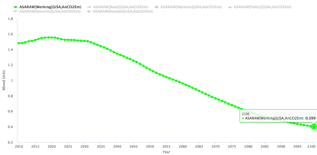
Cummulative change in carbon emissions, percent (billion tons), 2010-2100
TO DO: EXTRACT ANNUAL DATA POINTS
Src:
International Futures. Accessed August 22, 2016.
“Advanced Sustainability Analysis — USA, Working File”
The Pardee Center. University of Denver.
*
More data on carbon emissions can be found under the Energy Mix blog post.
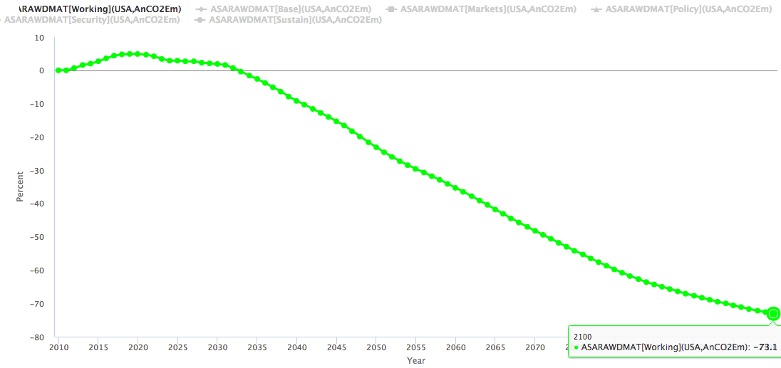
Water Use
Water use (cubic kilometers), cumulative change in raw values, percent, 2010-2100 (via the Advanced Sustainability table):
TO DO: EXTRACT ANNUAL DATA POINTS
Src:
International Futures. Accessed August 22, 2016.
“Advanced Sustainability Analysis — USA, Working File”
The Pardee Center. University of Denver.
Mining
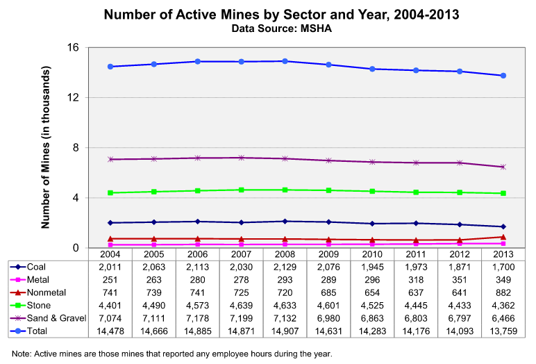
src:
CDC. Accessed August 24, 2016.
“Number of Active Mines by Sector and Year, 2004-2013.”
Statistics: All Mining
citing:
Mine Safety and Health Administration (MSHA)
TO DO: CONTACT MSHA TO CONFIRM SOURCE, AND INQUIRE ABOUT OLDER DATA.
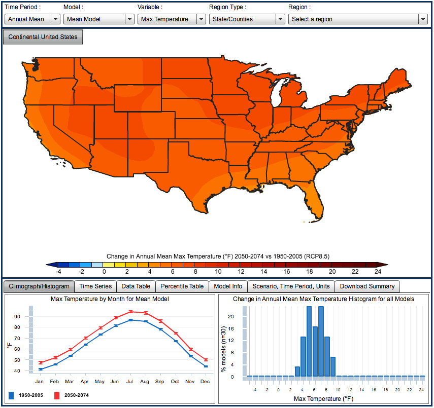
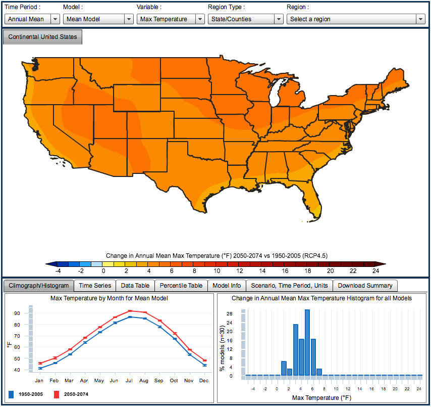
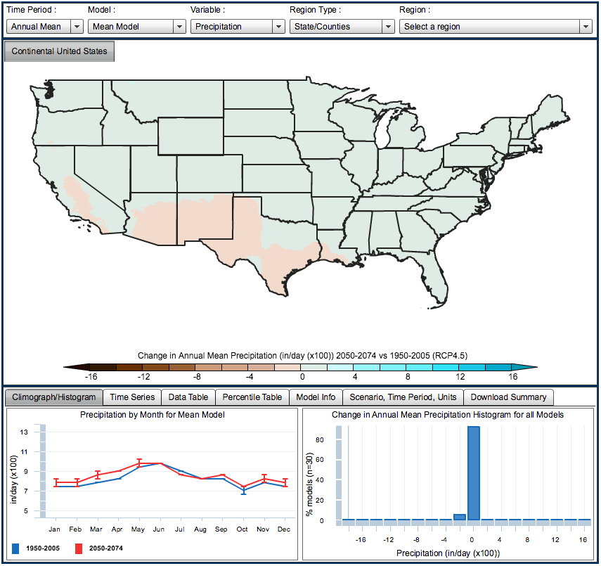
Climate Change
In 2013, NASA released climate projection data through 2099 for the continental United States that is being used to quantify climate risks to the nation’s agriculture, forests, rivers and cities.
The excerpts below shows the change for the 1950-2005 historic period versus the 2050-2074 forecast period. Max temperatures are trending up, precipitation is staying about the same, snow pack is trending down (dramatically in the Western mountains), and water stored in the soil column is trending down.
Excerpts:
Max Temperatures – High Emissions Scenario (RCP8.5)
Max Temperatures – Low Emissions Scenario (RCP4.5)
Precipitation — Low Emissions
Snow Water Equivalent — Low Emissions
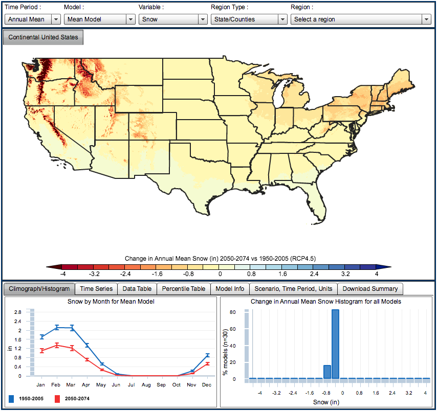
(Snow Water Equivalent — the liquid water stored in the snowpack)
Soil Water Storage – Low Emissions
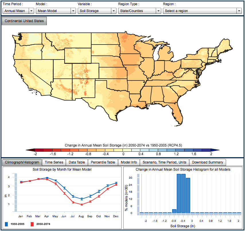
(Soil water storage: the water stored in the soil column)
src:
USGS. Accessed August 24, 2016.
“National Climate Change Viewer.”
NASA NEX DCP30 National Climate Change Viewer
The full NEX-DCP30 dataset includes 33 climate models for historical and 21st century simulations for four Representative Concentration Pathways (RCP) greenhouse gas (GHG) emission scenarios developed for AR5. … We include 30 of the 33 models in the viewer that have both RCP4.5 and RCP8.5 data; the remaining two scenarios, RCP2.6 and RCP6, are available in the NEX-DCP30 data set.
The NCCV allows the user to visualize projected changes in climate (maximum and minimum air temperature and precipitation) and the water balance (snow water equivalent, runoff, soil water storage and evaporative deficit) for any state, county and USGS Hydrologic Unit (HUC).
To create a manageable number of permutations for the viewer, we averaged the climate and water balance data into four climatology periods: 1950–2005, 2025–2049, 2050–2074, and 2075–2099.
src:
USGS. May 2014.
“U.S. Geological Survey – National Climate Change Viewer: Tutorial and Documentation.”
*
The National Climate Assessment (NCA), conducted by the U.S. Global Change Research Program, aggregates a mix of historic quantitative data, data projections, and qualitative descriptions of the impacts of the climate change trends that are being seen and are most likely to continue. Impacts on seven sectors are described: human health, water, energy, transportation, agriculture, forests, and ecosystems.
Citations are provided in-context below. The source information for the NCA report is at the very bottom.
Excerpts:
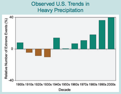
One measure of heavy precipitation events is a two-day precipitation total that is exceeded on average only once in a 5-year period, also known as the once-in-five year
event. As this extreme precipitation index for 1901-2012 shows, the occurrence of such events has become much more common in recent decades. Changes are compared to the period 1901-1960, and do not include Alaska or Hawai‘i. (Figure source: adapted from Kunkel et al. 2013 (7)).
p.25
7. K. E. Kunkel, et al. 2013.
“Monitoring and understanding trends in extreme storms: State of knowledge.”
Bulletin of the American Meteorological Society, 94.
Past and Projected Changes in Global Sea Level:
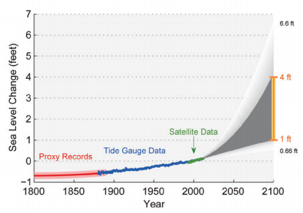
Figure shows estimated, observed, and possible amounts of global sea level rise from 1800 to 2100, relative to the year 2000. Estimates from proxy data (4) (for example, based on sediment records) are shown in red (1800-1890, pink band shows uncertainty), tide gauge data in blue for 1880-2009 (5), and satellite observations are shown in green from 1993 to 2012 (6). The future scenarios range from 0.66 feet to 6.6 feet in 2100 (7). These scenarios are not based on climate model simulations, but rather reflect the range of possible scenarios based on other kinds of scientific studies. The orange line at right shows the currently projected range of sea level rise of 1 to 4 feet by 2100, which falls within the larger risk-based scenario range. The large projected range reflects uncertainty about how glaciers and ice sheets will react to the warming ocean, the warming atmosphere, and changing winds and currents. As seen in the observations, there are year-to-year variations in the trend. (Figure source: Adapted from Parris et al. 2012 (7), with contributions from NASA Jet Propulsion Laboratory).
p.30
4. A. C. Kemp, et al. 2011.
“Climate related sea-level variations over the past two millennia.”
Proceedings of the National Academy of Sciences, 108, 11017-11022.
5. J. A. Church, et al. 2011.
“Sea-level rise from the late 19th to the early 21st century.”
Surveys in Geophysics, 32, 585-602.
6. R. S. Nerem, et al. 2010.
“Estimating mean sea level change from the TOPEX and Jason altimeter missions.”
Marine Geodesy, 33, 435-446.
Article is behind a paywall. Might be able to get even more current data from Nerem’s website.
7. A. Parris, et al. 2012
“Global Sea Level Rise Scenarios for the United States National Climate Assessment.”
NOAA Tech Memo OAR CPO-1, 37 pp. National Oceanic and Atmospheric Administration.
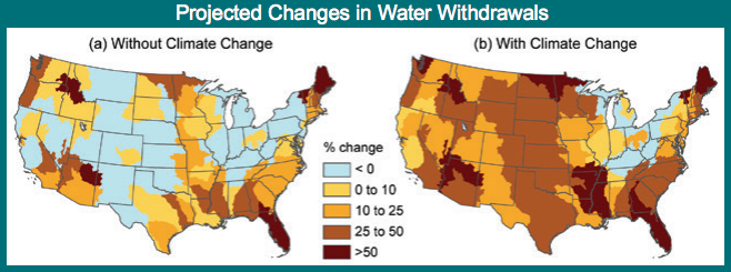
The effects of climate change, primarily associated with increasing temperatures and potential evapotranspiration, are projected to significantly increase water demand across most of the United States. Maps show percent change from 2005 to 2060 in projected demand for water assuming (a) change in population and socioeconomic conditions consistent with the A1B emissions scenario (increasing emissions through the middle of this century, with gradual reductions thereafter), but with no change in climate, and (b) combined changes in population, socioeconomic conditions, and climate according to the A1B emissions scenario. (Figure source: Brown et al. 2013 (4).)
p.43
4. T. C. Brown, et al. 2013.
“Projecting fresh water withdrawals in the United States under a changing climate.”
Water Resources Research, 49, 1259-1276/
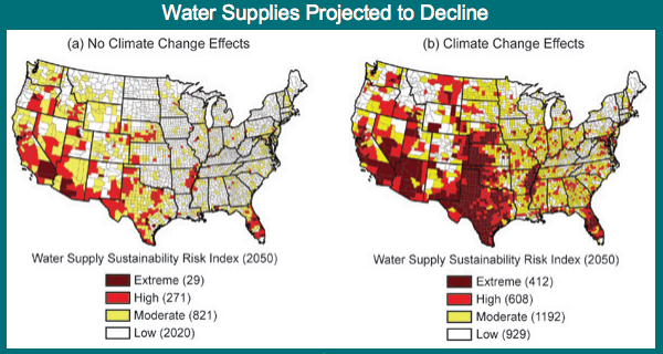
Climate change is projected to reduce water supplies in some parts of the country. This is true in areas where precipitation is projected to decline, and even in some areas where precipitation is expected to increase. Compared to 10% of counties today, by 2050, 32% of counties will be at high or extreme risk of water shortages. Numbers of counties are in parentheses in key. Projections assume continued increases in greenhouse gas emissions through 2050 and a slow decline thereafter (A1B scenario). (Figure source: Reprinted with permission from Roy et al. 2012 (7). Copyright American Chemical Society).
p.44
7. S. B. Roy, et al. 2012.
“Projecting water withdrawal and supply for future decades in the U.S. under climate change scenarios.”
Environmental Science & Technology, 46, 2545−2556.
Key Climate Variables Affecting Agricultural Productivity
Frost-free season is projected to lengthen across much of the nation. Taking advantage of the increasing length of the growing season and changing planting dates could allow planting of more diverse crop rotations, which can be an effective adaptation strategy.
The annual maximum number of consecutive dry days (less than 0.01 inches of rain) is projected to increase, especially in the western and southern parts of the nation, negatively affecting crop and animal production. The trend toward more consecutive dry days and higher temperatures will increase evaporation and add stress to limited water resources, affecting irrigation and other water uses.
Hot nights are defined as nights with a minimum temperature higher than 98% of the minimum temperatures between 1971 and 2000. Such nights are projected to increase throughout the nation. High nighttime temperatures can reduce grain yields and increase stress on animals, resulting in reduced rates of meat, milk, and egg production.
p.47
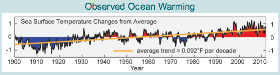
Sea surface temperatures for the ocean surrounding the U.S. and its territories have risen by more than 0.9°F over the past century. (Figure source: adapted from Chavez et al. 2011 (3)).
p.58
3. F. P. Chavez, et al. 2011.
“Marine primary production in relation to climate variability and change.”
Annual Review of Marine Science, 3, 227-260.
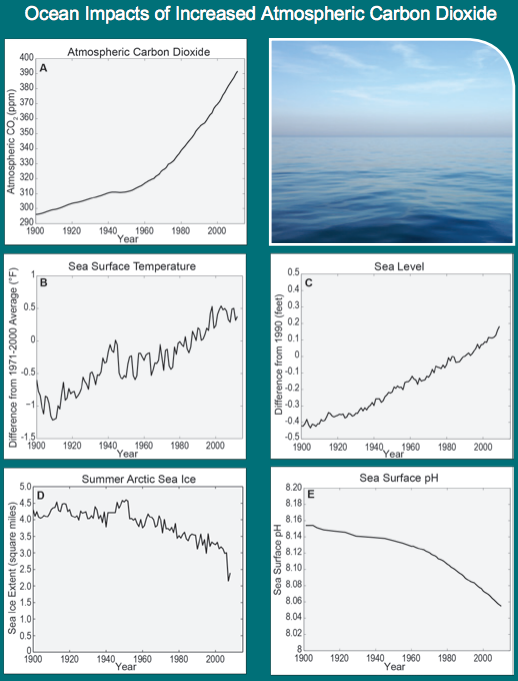
As heat-trapping gases, primarily carbon dioxide (CO2) (panel A), have increased over the past decades, not only has air temperature increased worldwide, but so has the ocean surface temperature (panel B). The increased ocean temperature, combined with melting of glaciers and ice sheets on land, is leading to higher sea levels (panel C). Increased air and ocean temperatures are also causing the continued, dramatic decline in Arctic sea ice during the summer (panel D). Additionally, the ocean is becoming more acidic as increased atmospheric CO2 dissolves into it (panel E). (CO2 data from Etheridge 2010, Tans and Keeling 2012, and NOAA NCDC 2012; SST data from NOAA NCDC 2012 and Smith et al. 2008; Sea level data from CSIRO 2012 and Church and White 2011; Sea ice data from University of Illinois 2012; pH data from Doney et al. 2012 (4,5)).
p.59
4. D. M. Etheridge, et al. 2010.
“Law Dome Ice Core 2000-Year CO2, CH4, and N2O Data, IGBP PAGES/World Data Center for Paleoclimatology.”
Data Contribution Series #2010-070. NOAA/NCDC Paleoclimatology Program, Boulder, CO.
CSIRO. 2012.
“The Commonwealth Scientific and Industrial Research Organisation.”
J. A. Church and N. J. White. 2011.
“Sea-level rise from the late 19th to the early 21st century.”
Surveys in Geophysics, 32, 585-602.
University of Illinois. 2012.
“Sea Ice Dataset”
University of Illinois, Department of Atmospheric Sciences.
S. C. Doney, et al. 2012.
“Climate change impacts on marine ecosystems.”
Annual Review of Marine Science, 4, 11-37.
5. P. Tans and R. Keeling. 2012.
“Trends in Atmospheric Carbon Dioxide, Full Mauna Loa CO2 Record.”
NOAA’s Earth System Research Laboratory.
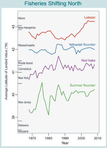
Ocean species are shifting northward along U.S. coastlines as ocean temperatures rise. As a result, over the past 40 years, more northern ports have gradually increased their landings of four marine species compared to earlier landings. While some species move northward out of an area, other species move in from the south. This kind of information can inform decisions about how to adapt to climate change. Such adaptations take time and have costs, as local knowledge and equipment are geared to the species that have long been present in an area. (Figure source: adapted from Pinsky and Fogerty 2012 (19)).
p.61
19. M. L. Pinsky and M. Fogarty. 2012.
“Lagged social-ecological responses to climate and range shifts in fisheries.”
Climatic Change, 115, 883-891.
src:
Jerry M. Melillo, et al. May 2014.
“Highlights of Climate Change Impacts in the United States: The Third National Climate Assessment.”
U.S. Global Change Research Program.
TO DO: EXTRACT DATA FROM SOURCES
